How Differentiation Works in Computers?

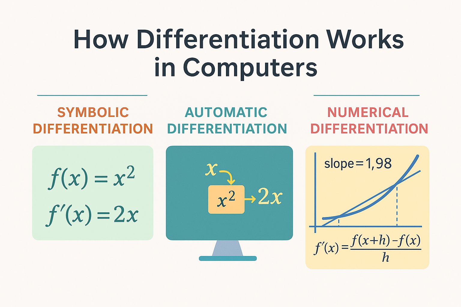
Table of Contents

1. Introduction
2. What is Differentiation?
3. Symbolic Differentiation
4. Numerical Differentiation
5. Automatic Differentiation
6. Summary
7. References

How It Started?

It all started when I was watching the YouTube video on Finding The Slope Algorithm (Forward Mode Automatic Differentiation) by Computerphile:

In this video, Mark Williams demonstrates Forward Mode Automatic Differentiation and explains how it addresses the limitations of traditional methods like Symbolic and Numerical Differentiation. The video also introduces the concept of Dual Numbers and shows how they can be efficiently used to compute the gradient of a function at any point.

Before diving into how computers do it, let’s quickly revisit what differentiation actually means.

Differentiation

In mathematics, the derivative is a fundamental tool that quantifies the sensitivity to change of a function's output with respect to its input. The derivative of a function of a single variable at a chosen input value, when it exists, is the slope of the tangent line to the graph of the function at that point. The process of finding a derivative is called differentiation.

Mathematical Definition

A function of a real variable \( f(x) \) is differentiable at a point \( a \) of its domain, if its domain contains an open interval containing \( ⁠a \)⁠, and the limit \( L \) exists.

$$ L = \lim_{h \to 0} \frac{f(a + h) - f(a)}{h} $$

Why We Calculate Derivatives?

Derivatives are a fundamental concept in calculus with many practical use cases across science, engineering, economics, and computer science. They measure how a quantity changes in response to a small change in another, commonly called "rate of change".

Think of a derivatives as answering:

"If I nudge the input just a little, how much does the output change?"

This makes derivatives crucial wherever change, sensitivity, or optimization is important. Some important applications include:

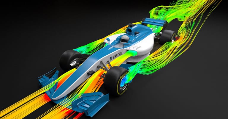
1. CFD (Computational Fluid Dynamics) 🌊: Simulates fluid flow by solving Navier–Stokes equations using partial derivatives of velocity, pressure, and density. These derivatives capture how small changes propagate, enabling realistic real-time simulations of smoke, fire, and airflow.

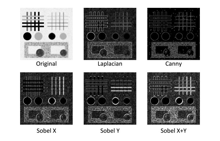
2. Image Processing & Edge Detection 🖼️: Image processing uses derivatives like Sobel filters and Laplacians to detect edges by identifying rapid changes in pixel intensity. This helps highlight boundaries for applications in computer vision and object recognition.

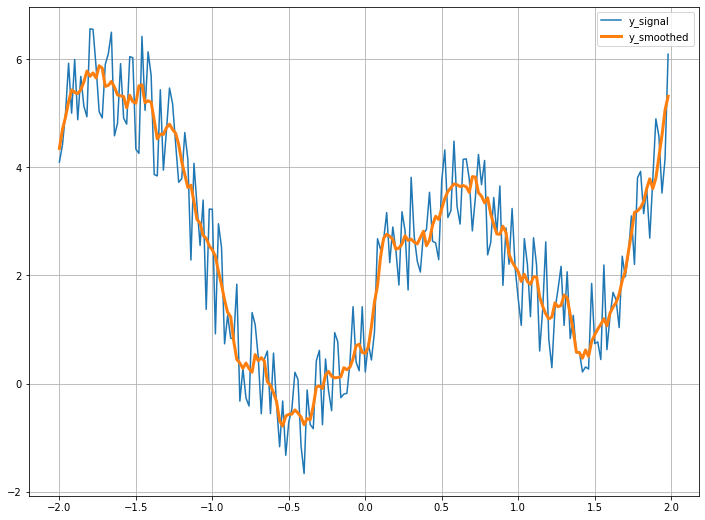
3. Signal Smoothing & Filtering 📡: Derivatives detect sudden spikes or noise in audio and sensor data, enabling smoothing and feedback control. This improves performance in applications like music processing, GPS filtering, and motion stabilization.

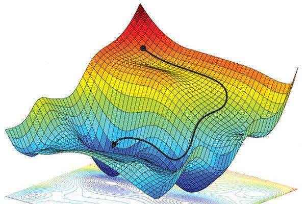
4. Machine Learning & AI 🧠: In machine learning, derivatives guide gradient descent by showing how to adjust weights to minimize loss. Backpropagation uses these derivatives to efficiently update neural network parameters during training.

Differentiation Methods

When it comes to differentiating with a computer, our first instinct is often the method we learned in high school, using known rules for common functions and applying them step by step. Let’s take a closer look at how that works!

1. Symbolic Differentiation

Symbolic differentiation relies on the fundamental definition of a derivative which is taking the limit of the difference quotient. After establishing the derivatives of basic functions, we can systematically apply differentiation rules to compute the derivatives of more complex expressions.

$$ \boxed{L = \lim_{h \to 0} \frac{f(a + h) - f(a)}{h}} $$

Let’s calculate it for a simple function: \( f(x)=x^n \)

$$ \displaylines{\begin{align} f(x) &= x^n \\ f'(x) &= \lim_{h \to 0} \frac{f(x+h) - f(x)}{h} \\ &= \lim_{h \to 0} \frac{(x + h)^n - x^n}{h}\end{align}} $$

Now apply the Binomial Theorem:

$$ (x + h)^n = x^n + n x^{n-1} h + \frac{n(n-1)}{2!} x^{n-2} h^2 + \cdots + h^n $$

Substitute this back into the limit:

$$ \displaylines{\begin{align}f'(x) &= \lim_{h \to 0} \frac{x^n + nx^{n-1}h + \frac{n(n-1)}{2!}x^{n-2}h^2 + \cdots + h^n - x^n}{h} \\ &= \lim_{h \to 0} \frac{nx^{n-1}h + \frac{n(n-1)}{2!}x^{n-2}h^2 + \cdots + h^n}{h} \\ &= \lim_{h \to 0} \left(nx^{n-1} + \frac{n(n-1)}{2!}x^{n-2}h + \cdots + h^{n-1}\right) \\ &= nx^{n-1}\end{align}} $$

Using the power rule from symbolic differentiation, the derivative is:

$$ \frac{d}{dx} x^n = n x^{n-1} $$

This rule is one of the foundational results and forms the basis for differentiating more complex expressions built from powers of \(x\). You’ve probably seen a sheet that lists differentiation rules formulas like this:

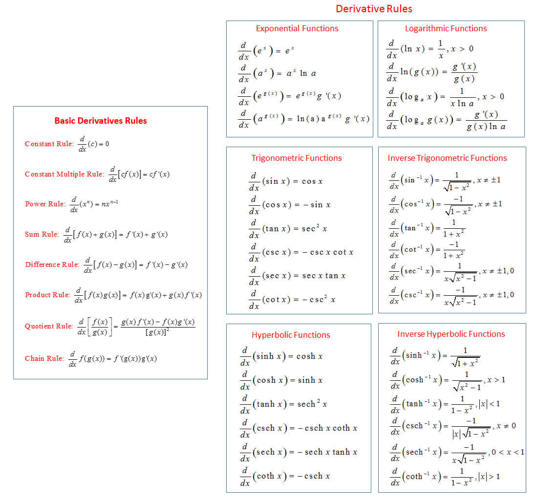
By breaking a complex function into smaller components and systematically applying basic rules such as the power, product, and chain rules you can compute the derivative of complex functions step-by-step.

We can implement this in any programming language by defining the fundamental rules and using them to compute derivatives. However, in Python, this functionality is already available through the sympy library. Let’s look at an example:

import sympy as sp

x = sp.Symbol("x")

f = x**2 + sp.sin(x)
f_prime = sp.diff(f, x)

print("f(x):", f)
print("f'(x):", f_prime)

# Substitute x = π
value = f_prime.subs(x, sp.pi)
# Evaluate the numeric value
numeric_value = value.evalf()
print(f"f'(π)={value}={numeric_value}")

Output

f(x): x**2 + sin(x)
f'(x): 2*x + cos(x)
f'(π)=-1 + 2*pi=5.28318530717959

While symbolic differentiation provides the exact mathematical expression for a function's rate of change, this elegance often falls short in real-world applications. What if your function isn't a neat equation, but rather a stream of experimental data or a "black-box" algorithm?

In these common scenarios, symbolic methods are simply unfeasible. This is precisely where numerical differentiation comes into picture. By approximating the derivative using discrete function values, it allows us to analyze the behavior of functions derived from empirical observations, complex simulations, or even cutting-edge machine learning models, areas where symbolic methods can't reach.

2. Numerical Differentiation

Numerical differentiation is the process of approximating the derivative of a function using its values at discrete points, rather than deriving an exact symbolic expression. It's used when a function's formula is unknown, too complex, or only available as data.

The simplest method used for numerical differentiation is finite difference approximations.

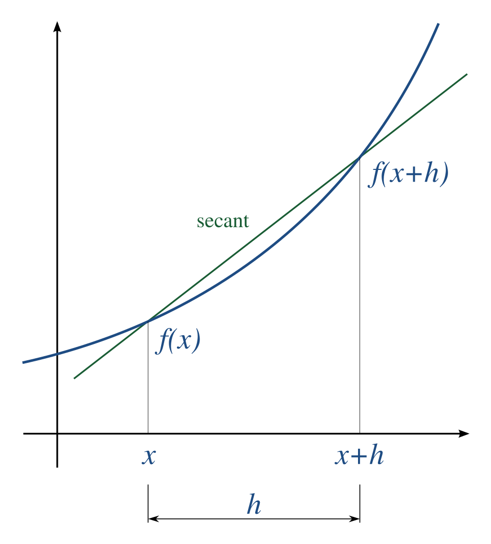
A simple two-point estimation is to compute the slope of a nearby secant line through the points \( (x, f(x)) \) and \( (x + h, f(x + h)) \). Choosing a small number \( h \), \( h \) represents a small change in \( x \), and it can be either positive or negative. The slope of this line is

$$ {\displaystyle {\frac {f(x+h)-f(x)}{h}}.} $$

This expression is Newton's difference quotient (also known as a first-order divided difference).

The slope of this secant line differs from the slope of the tangent line by an amount that is approximately proportional to \( h \). As \( h \) approaches zero, the slope of the secant line approaches the slope of the tangent line. Therefore, the true derivative of f at x is the limit of the value of the difference quotient as the secant lines get closer and closer to being a tangent line:

$$ {\displaystyle f'(x)=\lim _{h\to 0}{\frac {f(x+h)-f(x)}{h}}.} $$

We can easily implement numerical differentiation for any function. Let's look at the Python implementation for this:

import math

def f(x):
    return math.sin(x)

def f_dash(f, x, dx):
    return (f(x + dx) - f(x)) / dx

x = math.pi / 4
true_derivative = math.cos(x)
print("True Derivative: ", true_derivative)
print("Numerical Derivative: ", f_dash(f, x, dx=0.0001))

Output

True Derivative:  0.7071067811865476
Numerical Derivative:  0.7070714246693033

Another two-point formula is to compute the slope of a nearby secant line through the points \( (x − h, f(x − h)) \) and \( (x + h, f(x + h)) \). The slope of this line is

$$ {\displaystyle {\frac {f(x+h)-f(x-h)}{2h}}.} $$

This formula is known as the Symmetric difference quotient. In this case the first-order errors cancel, so the slope of these secant lines differ from the slope of the tangent line by an amount that is approximately proportional to \( h^{2} \). Hence for small values of \( h \) this is a more accurate approximation to the tangent line than the one-sided estimation.

Let's implement this in Python:

import math

def f(x):
    return math.sin(x)

def f_dash_symetric(f, x, dx):
    return (f(x + dx) - f(x - dx)) / (2 * dx)

x = math.pi / 4
true_derivative = math.cos(x)
print("True Derivative: ", true_derivative)
print("Numerical Derivative: ", f_dash_symetric(f, x, dx=0.0001))

Output

True Derivative:  0.7071067811865476
Numerical Derivative:  0.70710678000796

Numerical differentiation is quick and easy to implement, especially when an explicit formula for the derivative is unavailable or the function is defined only through data points.

However, it comes with certain limitations. The results are highly sensitive to the choice of step size, too large and the approximation is inaccurate; too small and rounding errors dominate due to floating-point precision limits. The following diagram represents this tradeoff and the sweet-spot for accurate calculations.

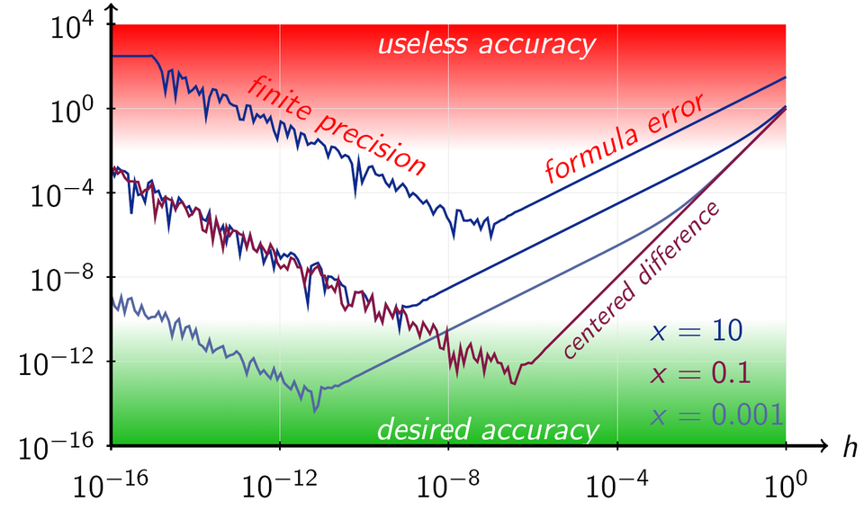
Let's try to replicate the results by calculating this error and plotting using Matplotlib:

import math
import matplotlib.pyplot as plt

def f(x):
    return math.sin(x)

def f_dash(f, x, dx):
    # Newton's difference
    return (f(x + dx) - f(x)) / dx

def f_dash_symetric(f, x, dx):
    # Symmetric difference
    return (f(x + dx) - f(x - dx)) / (2 * dx)

# Point at which to differentiate
x = math.pi / 4
true_derivative = math.cos(x)

# dx values
dx_values = [2 ** (-i) for i in range(1, 50)]

# Compute numerical derivatives and errors
errors_newton = [abs(f_dash(f, x, dx) - true_derivative) for dx in dx_values]
errors_symmetric = [
    abs(f_dash_symetric(f, x, dx) - true_derivative) for dx in dx_values
]

# Plotting
plt.figure(figsize=(16, 9))
plt.loglog(dx_values, errors_newton, marker="o", label="Newton's Difference")
plt.loglog(dx_values, errors_symmetric, marker="s", label="Symmetric Difference")
plt.xlabel("dx (step size)")
plt.ylabel("Absolute Error")
plt.title("Error Comparison of Numerical Differentiation Methods at x = π/4")
plt.grid(True, which="both", ls="--")
plt.legend()
plt.show()

Output:

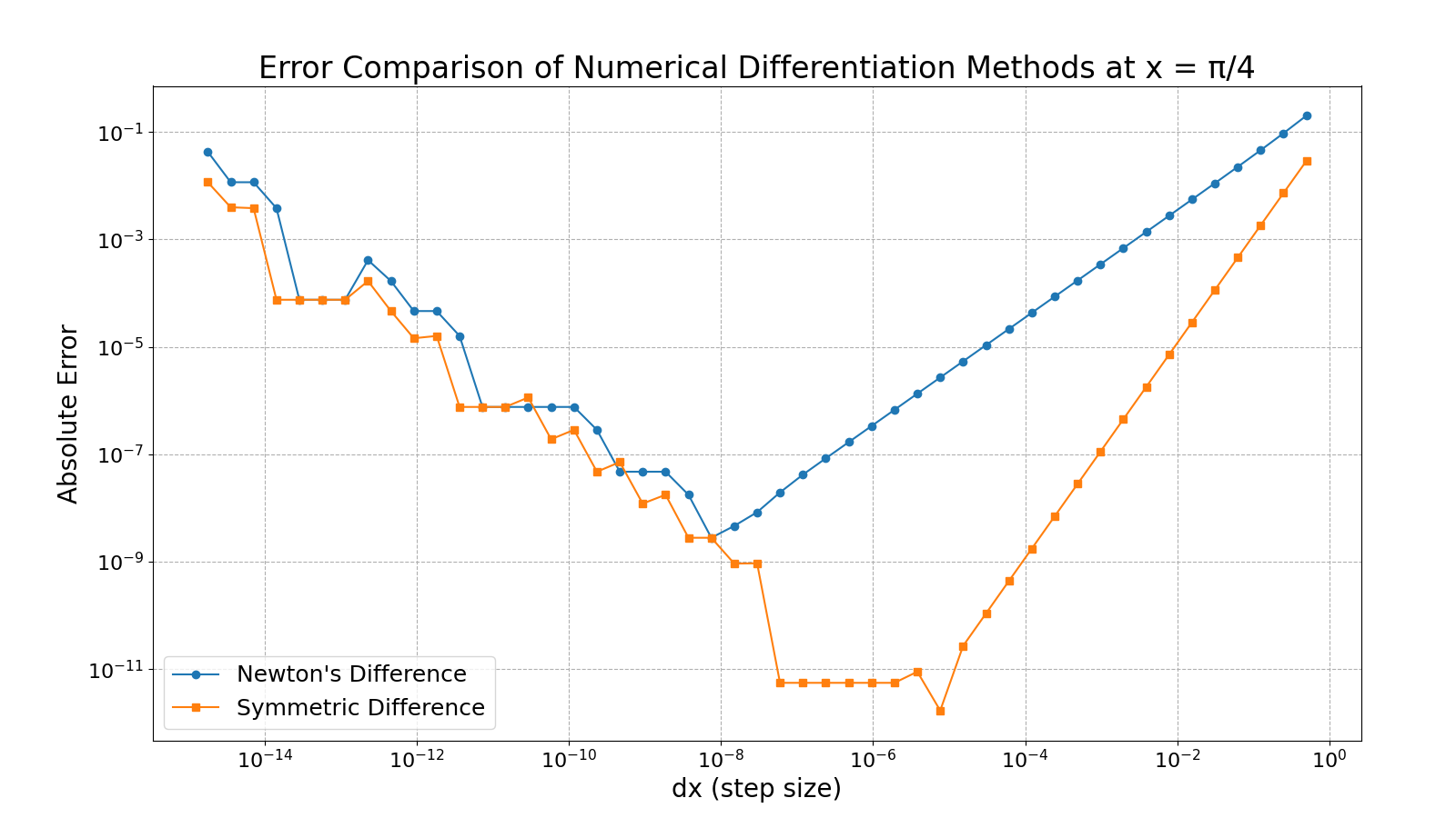
We observe a similar pattern as in the previous diagram, highlighting how numerical differentiation is sensitive to step size. Apart from this it also tends to amplify any noise in the data, making it unreliable for real-world measurements or simulations with fluctuations. Additionally, it provides only pointwise estimates and does not yield a general formula, limiting its usefulness in analytical studies or symbolic manipulation.

3. Automatic Differentiation

Now let’s look into automatic differentiation, a powerful technique that computes exact derivatives by breaking down functions into elementary operations and applying the chain rule systematically.

Unlike numerical differentiation, it avoids rounding and truncation errors, and unlike symbolic differentiation, it scales well with complex functions. Both of these classical methods have problems with calculating higher derivatives, where complexity and errors increase. This makes automatic differentiation especially powerful in machine learning and scientific computing where accurate gradients are essential.

Auto-differentiation is thus neither numeric nor symbolic, nor is it a combination of both. It is also preferable to ordinary numerical methods: In contrast to the more traditional numerical methods based on finite differences, auto-differentiation is 'in theory' exact, and in comparison to symbolic algorithms, it is computationally inexpensive.

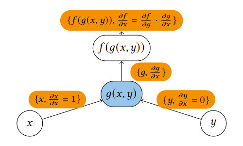
Automatic Differentiation (AD) is a structured, algorithmic method for efficiently computing derivatives by systematically applying the chain rule. At its core, AD relies on breaking down the differentiation process using the chain rule for composite functions.

For a nested function:

$$ y = f(g(h(x))) = f(g(h(w_0))) = f(g(w_1)) = f(w_2) = w_3 $$

with intermediate variables:

$$ \displaylines{\begin{align}w_0 &= x \\ \quad w_1 &= h(w_0) \\ \quad w_2 &= g(w_1) \\ \quad w_3 &= f(w_2) = y\end{align}} $$

the chain rule gives:

$$ \frac{\partial y}{\partial x} = \frac{\partial y}{\partial w_2} \cdot \frac{\partial w_2}{\partial w_1} \cdot \frac{\partial w_1}{\partial x} = \frac{\partial f(w_2)}{\partial w_2} \cdot \frac{\partial g(w_1)}{\partial w_1} \cdot \frac{\partial h(w_0)}{\partial x}. $$

Types of Automatic Differentiation

Usually, two distinct modes of automatic differentiation are presented:

• Forward accumulation (also called bottom-up, forward mode, or tangent mode)
• Reverse accumulation (also called top-down, reverse mode, or adjoint mode)

Forward accumulation specifies that one traverses the chain rule from inside to outside (that is, first compute \( \partial w_{1}/\partial x \) and then \( \partial w_{2}/\partial w_{1} \) and lastly \( \partial y/\partial w*{2}\) ), while reverse accumulation traverses from outside to inside (first compute \( \partial y/\partial w_{2} \) and then \( \partial w_{2}/\partial w_{1} \) and lastly \( \partial w_{1}/\partial x\) ).

Forward-mode Automatic Differentiation

In forward accumulation AD, one first fixes the independent variable with respect to which differentiation is performed and computes the derivative of each sub-expression recursively. In a pen-and-paper calculation, this involves repeatedly substituting the derivative of the inner functions in the chain rule:

Let the chain of intermediate variables be:

$$ w_0 = x, \quad w_1 = f_1(w_0), \quad w_2 = f_2(w_1), \quad \dots, \quad w_n = f_n(w_{n-1}) = y $$

Then, by the chain rule, the derivative of \( y \) with respect to \( x \) is:

$$ \frac{dy}{dx} = \frac{dw_n}{dw_{n-1}} \cdot \frac{dw_{n-1}}{dw_{n-2}} \cdot \dots \cdot \frac{dw_1}{dw_0} $$

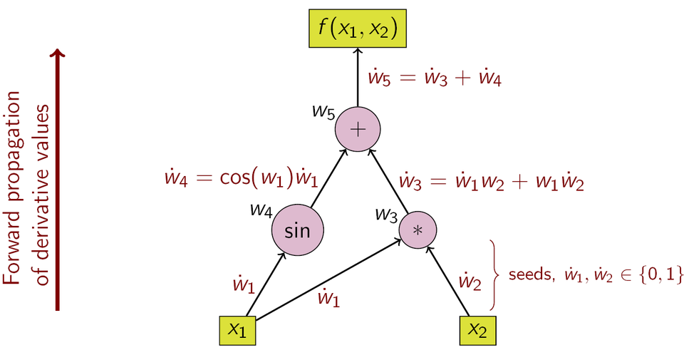
In forward mode automatic differentiation, we compute both the value and the derivative of each intermediate variable \( w_i \) in a single forward pass:

$$ \text{For each } i = 1 \text{ to } n: \displaylines{\begin{align} w_i &= f_i(w_{i-1}) \\ \dot{w_i} &= f_i'(w_{i-1}) \cdot \dot{w}_{i-1} \end{align}} $$

where \( \dot{w}_i = \frac{dw_i}{dx} \) denotes the derivative of \( w_i \) with respect to the fixed input variable \( x \).

We will now look at the dual number-based implementation of forward mode automatic differentiation, which allows us to compute derivatives alongside function evaluations in a natural and efficient way.

Dual Numbers

Definition

Dual numbers extend the real numbers by introducing a new element \( \varepsilon \) (epsilon) such that:

$$ \varepsilon^2 = 0, \quad \varepsilon \ne 0 $$

Any dual number has the form:

$$ a + b\varepsilon $$

where:

• \( a \) and \( b \) are real numbers,
• \( \varepsilon \) is a \( \textit{nilpotent} \) element (i.e., its square is zero).

Arithmetic

Let \( x = a + b\varepsilon \), \( y = c + d\varepsilon \).

1. Addition:

   $$ x + y = (a + c) + (b + d)\varepsilon $$

2. Multiplication:

   $$ x \cdot y = (a + b\varepsilon) * (c + d\varepsilon) = ac + (ad + bc)\varepsilon \quad \text{(since } \varepsilon^2 = 0 \text{)} $$

Automatic Differentiation

Consider the Taylor series expansion of a function \( f(x) \) evaluated at the point \( x+\varepsilon \):

$$ f(x+\varepsilon) = f(x) + f'(x)\varepsilon + \frac{1}{2}f''(x)\varepsilon^2 + \cdots $$

Due to the property of dual numbers where \( \varepsilon^2 = 0 \), therefore \( \varepsilon_1^k = 0 \) for all \( k > 1 \), all higher-order terms in the expansion vanish. Consequently, the Taylor series reduces to:

$$ f(x+\varepsilon) = f(x) + \varepsilon f'(x) $$

This truncation occurs because the dual number property eliminates all polynomial terms of degree two and higher, leaving only the linear approximation. Therefore, if you evaluate a function \( f(a + b\varepsilon) \), you get:

$$ f(a + b\varepsilon) = f(a) + b f'(a)\varepsilon $$

This means you can compute both \( f(a) \) and \( f'(a) \) in one pass, a powerful technique in machine learning and scientific computing. Let's implement the dual numbers in Python:

import math


class Dual:
    def __init__(self, real, dual):
        self.real = real
        self.dual = dual

    def __str__(self):
        return f"{self.real}+{self.dual}ε"

    def __add__(self, other):
        if isinstance(other, Dual):
            real = self.real + other.real
            dual = self.dual + other.dual
            return Dual(real, dual)
        return Dual(self.real + other, self.dual)

    __radd__ = __add__

    def __mul__(self, other):
        if isinstance(other, Dual):
            real = self.real * other.real
            dual = self.real * other.dual + self.dual * other.real
            return Dual(real, dual)
        return Dual(self.real * other, self.dual * other)

    __rmul__ = __mul__


d1 = Dual(3, 2)
d2 = Dual(4, 5)
print(f"d1: {d1}, d2: {d2}")
print("d1+d2 =", d1 + d2)
print("d1*d2 =", d1 * d2)

Output

d1: 3+2ε, d2: 4+5ε
d1+d2 = 7+7ε
d1*d2 = 12+23ε

Before we move on to the implementation of differentiation using dual numbers, which is quite easy, we need to first implement another commonly used function: the power function.

Let \( x=a+bε \), and suppose you want to compute \( x^y \), considering two cases:

Case 1: \( y \in \mathbb{R} \) (a real exponent)

Let \( y = n \in \mathbb{R} \). Using the first-order Taylor expansion:

$$ x^n = (a + b\varepsilon)^n = a^n + n a^{n-1} b \varepsilon $$

Thus, the result is:

• Real part: \( a^n \)
• Dual part: \( n a^{n-1} b \)

Which gives:

real = self.real**other
dual = other * self.real ** (other - 1) * self.dual

Case 2: \( y = c + d\varepsilon \) (a dual exponent)

We use the identity:

$$ x^y = e^{y \cdot \ln x} $$

First compute:

$$ \ln x = \ln(a + b\varepsilon) = \ln a + \frac{b}{a} \varepsilon $$

Then:

$$ y \cdot \ln x = (c + d\varepsilon)(\ln a + \frac{b}{a} \varepsilon) = c \ln a + \left( d \ln a + \frac{c b}{a} \right) \varepsilon $$

Now exponentiate:

$$ e^{c \ln a + \left( d \ln a + \frac{c b}{a} \right) \varepsilon} = a^c + a^c \left( d \ln a + \frac{c b}{a} \right) \varepsilon $$

So:

• Real part: \( a^c \)
• Dual part: \( a^c \left( \frac{c b}{a} + d \ln a \right) \)

This gives:

real = self.real ** other.real
dual = real * (
(self.dual * other.real / self.real) + other.dual * math.log(self.real)
)

Now to calculate the derivative of a function, evaluating a function \( f \) at the dual number \( x + \varepsilon \), we get:

$$ f(x + \varepsilon) = f(x) + f'(x)\varepsilon $$

The real part is the value of the function, and the dual part gives the derivative. Hence, we can extract the derivative directly from the dual component. The derivative of \( f \) at a point \( x \) can be computed using:

def diff(f, x):
    return f(Dual(x, 1)).dual

Here, we construct the dual number \( x + 1 \cdot \varepsilon \). When \( f \) is evaluated on this dual number, it propagates the derivative information through all operations. The final .dual part gives us \( f'(x) \).

Now putting everything together we have:

import math


class Dual:
    def __init__(self, real, dual):
        self.real = real
        self.dual = dual

    def __str__(self):
        return f"{self.real}+{self.dual}ε"

    def __add__(self, other):
        if isinstance(other, Dual):
            real = self.real + other.real
            dual = self.dual + other.dual
            return Dual(real, dual)
        return Dual(self.real + other, self.dual)

    __radd__ = __add__

    def __mul__(self, other):
        if isinstance(other, Dual):
            real = self.real * other.real
            dual = self.real * other.dual + self.dual * other.real
            return Dual(real, dual)
        return Dual(self.real * other, self.dual * other)

    __rmul__ = __mul__

    def __pow__(self, other):
        if isinstance(other, (int, float)):
            real = self.real**other
            dual = other * self.real ** (other - 1) * self.dual
            return Dual(real, dual)
        elif isinstance(other, Dual):
            real = self.real**other.real
            dual = real * (
                (self.dual * other.real / self.real) + other.dual * math.log(self.real)
            )
            return Dual(real, dual)
        else:
            return NotImplemented


def diff(f, x):
    return f(Dual(x, 1)).dual

Let's try to find the derivative of a polynomial function using our implementation.

def f(x):
    return x**2 + 3 * x + 2

x = 5
print("f(x) = ", f(x))
print("f'(x) = ", diff(f, x))
print("f'(x) = ", 2 * x + 3)

Output

f(x) =  42
f'(x) =  13
f'(x) =  13

We can use similar approach to calculate the propagation of derivatives for trigonometric function like \( \sin(x) \) and \( \cos(x) \), where \( x \in \mathbb{D} \) (dual numbers). We use Taylor expansion and the chain rule to propagate derivatives through the dual part.

Sine Function

$$ \sin(x) = \sin(a + b\varepsilon) $$

Using first-order Taylor expansion:

$$ \sin(a + b\varepsilon) = \sin(a) + b\varepsilon \cdot \cos(a) $$

So, the result is:

$$ \text{real part: } \sin(a), \quad \text{dual part: } b \cos(a) $$

In code:

def sin(x):
    if isinstance(x, Dual):
        return Dual(math.sin(x.real), x.dual * math.cos(x.real))
    return math.sin(x)

Cosine Function

$$ \cos(x) = \cos(a + b\varepsilon) $$

Using Taylor expansion:

$$ \cos(a + b\varepsilon) = \cos(a) - b\varepsilon \cdot \sin(a) $$

So, the result is:

$$ \text{real part: } \cos(a), \quad \text{dual part: } -b \sin(a) $$

In code:

def cos(x):
    if isinstance(x, Dual):
        return Dual(math.cos(x.real), -x.dual * math.sin(x.real))
    return math.cos(x)

Let's test our implementation:

def f(x):
    return sin(x)

x = math.pi / 3
print("f(x) = ", f(x))
print("f'(x) = ", diff(f, x))
print("f'(x) = cos(x) = ", cos(x))

Output

f(x) =  0.8660254037844386
f'(x) =  0.5000000000000001
f'(x) = cos(x) =  0.5000000000000001

In summary, forward-mode automatic differentiation leverages dual numbers to elegantly propagate derivatives alongside values. By evaluating functions on dual inputs, we can compute exact derivatives with minimal changes to the original code, making this technique both efficient and easy to implement.

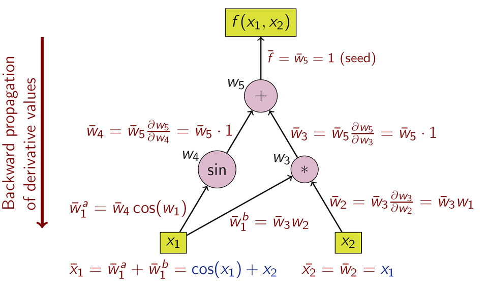
Reverse-mode Automatic Differentiation

It's worth noting that another powerful technique exists: reverse-mode automatic differentiation, which is more efficient when computing gradients of functions with many inputs and a single output like in deep learning. However, reverse mode requires building a computational graph and performing a backward pass, which adds complexity. We won’t cover reverse-mode here, as that would make this post significantly longer.

Wrapping Up

Differentiation is at the heart of optimization, and in today's machine learning and scientific computing workflows, automatic differentiation offers the best of both worlds: precision and efficiency.

We’ve seen how to go from symbolic and numerical methods to a more scalable and elegant solution, one that can be embedded directly in code with minimal overhead. Forward-mode using dual numbers provides an elegant way to compute derivatives by augmenting the real number system and propagating derivatives alongside values.

Different differentiation methods serve different needs depending on the context. Here’s a quick comparison of symbolic, numerical, and automatic differentiation to help you understand when to use which:

Method	Pros	Cons	Best for
Symbolic	Exact derivatives	Slow for complex functions	Math-heavy functions
Numerical	Simple to implement	Inaccurate, error-prone	Unknown/black-box functions
Automatic	Accurate and efficient	Harder to implement manually	ML, optimization problems

If you’ve come this far, thank you! I hope this post demystified how computers differentiate functions and how that knowledge translates into real-world applications.

Until next time, keep exploring, and keep differentiating 🧮🚀

References

1. Derivative - Wikipedia
2. Differentiation Rules
3. Numerical differentiation - Wikipedia
4. Automatic differentiation - Wikipedia
5. Dual Numbers for Arbitrary Order Automatic Differentiation

Stay Tuned

Hope you enjoyed reading this. Stay tuned for more cool stuff coming your way!