Measuring Distances using Rope

History of Length Measurement

The measurement of length has a long and varied history, dating back to ancient civilizations that developed standardized units to support trade, construction, and agriculture. The earliest recorded systems emerged in Mesopotamia and Egypt, where cubits—based on the length of a forearm—were commonly used. In Ancient Rome, the foot (based on the human foot) became a standard unit, while in Ancient India, the dhanus(bow), the krosha and the yojana were widely employed.

Early measuring methods for length were based on the use of human body parts. Lengths and width of fingers, thumbs, hands, hand spans, cubits and body spans seem to have been popular choices.

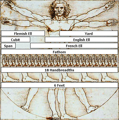
Using body parts for measurement, as was common in ancient times, posed several significant issues. The primary challenge was the lack of standardization, as body parts vary significantly between individuals. This lack of uniformity hindered large-scale projects and international trade, where consistency was crucial.

The advent of the metric system in France during the late 18th century revolutionized length measurement by introducing a universal system based on the meter. This system gradually became the global standard, promoting international coherence in science, industry, and commerce.

Enough of history, let's explore an interesting problem now.

The Explorer and the Rope

Once upon a time, a seasoned sea explorer found himself stranded on a remote island with nothing but a 10-meter rope and his wits. Far from civilization and stripped of his usual tools, he faced the daunting task of creating a reliable measurement system from scratch to build his ship to get back.

Suppose you are the explorer. How would you go about solving this problem?

Hint: Think about how you would measure distances like 20m, 25m, 32m, 41.5m etc.

Approach

Given a 10-meter rope, what's the distance we can measure right away?

Well, it is 10m and we can also measure distances that are multiples like 20m, 30m, 40m etc. 20 meters would be two rope lengths and so on. This approach is straightforward but limited in precision.

What about measuring distance like 25 meters?

If you want to measure a distance that isn't an exact multiple of your rope's length, you can divide the rope into smaller, equal sections to measure the remaining distance.

We can divide the rope in half by folding it giving us a measure of 5 meters and therefore we can now measure 25 meters:

$$D = 10 * 2 + 5$$

How about measuring distances like 8.5m, 12.25m?

We can further keep diving the rope in half to get the measure of 2.5m, 1.25m and so forth. But given these measures how can we accurately measure an arbitrary length like 23.426m?

Let's look at the mathematical representation of this problem to find out the answers.

Mathematical Representation

Let's represent the problem mathematically:

Variables:

• \( L \) = Full length of the rope
• \( D \) = Total distance to be measured
• \( n \) = Number of full lengths of the rope required to span most of the distance
• \( r \) = Remaining distance after using \( n \) full lengths of the rope

Algorithm:

1. Initial Step: Use Full Rope Length:

   $$ n = \left\lfloor \frac{D}{L} \right\rfloor $$

   The remaining distance \( r \) is:

   $$ r = D - n \cdot L $$

2. Iterative Approximation Process:

   Now by dividing the rope, we can measure distances like \( \frac{L}{2} \), \( \frac{L}{4} \), \( \frac{L}{8} \) and so forth.

   Let us represent the smaller divisions by \(l_i\) where:

   $$l_i = \frac{L}{2^i}$$

   Now, as \(0 \le r < L\) we can estimate \( r \) by using combinations of \(l_i\). Therefore,

   $$r_{approx} = \frac{L}{2} \pm \frac{L}{4} \pm \frac{L}{8} \pm \frac{L}{16} \cdots$$

   How can we be sure that this approximation covers the whole range?

   First, let us try to analyze the minimum and maximum values that \(r_{approx}\) can attain:

   The sum \( S \) of an infinite geometric series can be expressed as: $$S = \sum_{n=0}^{\infty} ar^n = \frac{a}{1 - r}$$

   where:

   • \( a \) is the first term,
   • \( r \) is the common ratio, and \( |r| < 1 \).

   The minimum value is attained when all following terms are negative i.e.

   $$ \displaylines{\begin{align} \min({r_{approx}}) &= \frac{L}{2} - \frac{L}{4} - \frac{L}{8} - \frac{L}{16} \cdots \\ &= \frac{L}{2} - \frac{L}{4}\sum_{n=0}^{\infty} 2^{-n} \\ &= \frac{L}{2} - \frac{L}{4}*\frac{1}{1 - \frac{1}{2}} \\ &= 0\end{align}} $$

   Similarly, the maximum value is attained when all following terms are positive i.e.

   $$ \displaylines{\begin{align} \max({r_{approx}}) &= \frac{L}{2} + \frac{L}{4} + \frac{L}{8} + \frac{L}{16} \cdots \\ &= \frac{L}{2} + \frac{L}{4}\sum_{n=0}^{\infty} 2^{-n} \\ &= \frac{L}{2} + \frac{L}{4}*\frac{1}{1 - \frac{1}{2}} \\ &= L\end{align}} $$

   The proof that that this approximation covers the whole range is left as an exercise for the reader. 😉

   Approximation:

   We start by approximating \( r \) as \( \frac{L}{2} \). Therefore:

   $$ r_0 = \frac{L}{2} $$

   For each iteration \( i \):

   • Divide the rope length by \( k_i = 2^{i+1} \): $$ l_i = \frac{L}{2^{i+1}} $$

   • Calculate the error \( ε \): $$ ε_i = r - r_i $$

   • Calculate the next direction to move on the number line \( m_{i+1} \): $$ m_{i+1} = \frac{{r - r_i}}{\left|{r - r_i}\right|} = \frac{{ε_i}}{\left|{ε_i}\right|} $$

   • The new approximation \( r_{i+1} \) becomes: $$ r_{i+1} = r_i + m_{i+1} \cdot l_{i+1} $$

   • If \( ε_i \) is small enough (i.e., less than the current precision threshold), stop the process.

     $$ r \approx \frac{L}{2} + \sum_{i=1}^{\text{max iterations}} m_i \cdot l_i $$

3. Sum the Total Distance:

   $$ D \approx n \cdot L + \frac{L}{2} + \sum_{i=1}^{\text{max iterations}} m_i \cdot l_i $$

Approximation Formula

$$ \boxed{D \approx n \cdot L + \frac{L}{2} + \sum_{i=1}^{\text{max iterations}} m_i \cdot l_i} $$

where:

• \( L \) is the length of the rope
• \( n = \left\lfloor \frac{D}{L} \right\rfloor \) is the number of full rope lengths
• \( l_i = \frac{L}{2^{i+1}} \) is the length of smaller ropes formed by successive halving
• \( m_i \) is the coefficient of length \( l_i \) and \( m_i \in \lbrace 1, -1\rbrace \) for \( i = 1, 2, \dots, k \)

Example:

Suppose you have a rope of length \( L = 8 \) meters, and you need to measure a distance \( D = 19 \) meters.

1. Step 1: Initial Full Lengths:

   $$ n = \left\lfloor \frac{11}{8} \right\rfloor = 2 $$

   The distance covered is \( 2 \cdot 8 = 16 \) meters.

   $$ r = 19 - 16 = 3 \text{ meters} $$

2. Step 2: Initial approximation:

   • Initial approximation: \( r_0 = \frac{8}{2} = 4 \) meters.

3. Step 2: First approximation:

   • Initial approximation: \( r_0 = \frac{8}{2} = 4 \) meters.
   • Error: \( ε_0 = r - r_0 = 3 - 4 = -1\)
   • Rope measure: \( l_1 = \frac{8}{4} = 2 \) meters.
   • Direction to move: \( m_1 = \frac{{ε_0}}{\left|{ε_0}\right|} = -1 \).
   • New approximation: \( r_1 = 4 + (-1)*2 = 2 \) meter.

4. Step 3: Second Approximation:

   • Previous approximation: \( r_1 = 2 \) meter.
   • Error: \( ε_1 = r - r_1 = 3 - 2 = 1\)
   • Rope length: \( l_2 = \frac{8}{8} = 1 \) meters.
   • Direction to move: \( m_2 = \frac{{ε_1}}{\left|{ε_1}\right|} = 1 \).
   • New approximation: \( r_2 = 2 + 1*1 = 3 \) meter.

5. Step 4: Halt Approximation:

   • Previous approximation: \( r_2 = 3 \) meter.
   • Error: \( ε_2 = r - r_2 = 3 - 3 = 0\)

   As the error is zero, we have successfully approximated the distance.

6. Step 5: Total Distance Approximation:

   $$ \displaylines{\begin{align}D &\approx 2 \cdot 8 + 4 + 2 \cdot -1 + 1 \cdot 1 \\ &= 16 + 4 - 2 + 1 \\ &= 19 \text{ meters}\end{align}} $$

Precision:

By halving the rope length at each step, you can continue this process until the remaining distance is negligible, providing an increasingly precise measurement. This method mirrors the binary search algorithm, where the solution space is progressively halved until the desired precision is reached.

This method allows you to measure distances more accurately using just the rope, without needing additional tools or scales.

Python Implementation

ERROR = 0.0001
MAX_ITERATIONS = 100


# distance < scale
def measure(distance, scale):
    iteration = 1
    y_prev = scale / 2

    if distance < ERROR:
        return distance, 0

    while iteration < MAX_ITERATIONS and abs(distance - y_prev) > ERROR:
        direction = 1 if (distance - y_prev) > 0 else -1
        y_next = y_prev + direction * (scale / pow(2, iteration + 1))
        iteration += 1
        y_prev = y_next

    return y_prev, iteration


def measure_repeated(distance, scale):
    full = int(distance / scale)
    remaining = distance - full * scale
    approx, iterations = measure(remaining, scale)
    return {"approximation": full * scale + approx, "iterations": full + iterations}

This code provides two main functions, measure and measure_repeated, which estimate values iteratively by measuring the distance in relation to a given scale. Here's a breakdown of how it works:

• measure: Uses an iterative approach with diminishing step sizes (halving each time) to approximate a given distance within a specified ERROR margin. It ensures that the approximation is as close as possible to the target within a reasonable number of iterations.

• measure_repeated: Enhances the measure function by handling larger distances that may consist of multiple full scale units plus a remainder. It efficiently breaks down the problem, approximates the remainder, and combines the results.

ERROR = 0.0001  # The allowable error threshold for stopping iterations
MAX_ITERATIONS = 100  # Maximum number of iterations to perform in the measurement

Usage Example:

scale = 10

print(measure(5, scale))
print(measure(4.9, scale))

print(measure_repeated(10, scale))
print(measure_repeated(3.75, scale))
print(measure_repeated(9.8, scale))

Let's look at the output of this approximation algorithm:

animesh@pop-os:~$ python -u "measure.py"
(5.0, 1)
(4.89990234375, 12)
{'approximation': 10, 'iterations': 1}
{'approximation': 3.75, 'iterations': 3}
{'approximation': 9.7999572, 'iterations': 16}

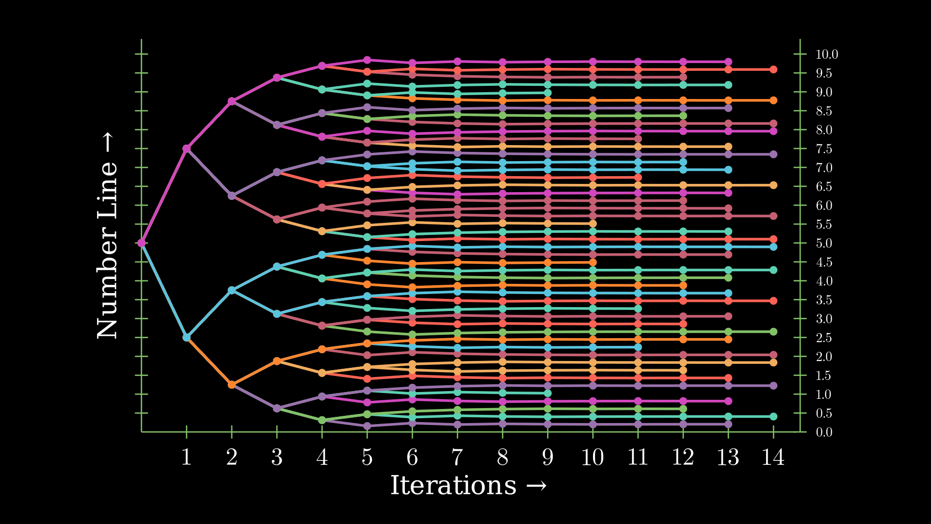
Visualization

Here's a visualization of this method created using Manim:

Convergence Analysis

In our initial approach, we repeatedly halved the rope length to achieve more precise measurements. But why didn’t we divide it by 3 or even 4 instead?

Let's take a look at the generalized version of this approximation:

Given:

• \( L \) is the initial length of the rope.
• \( \alpha \) is the scaling factor that determines how much the rope length is reduced at each step.
• \( D \) is the total distance you want to measure.

The process involves measuring the distance using the rope, then successively reducing the rope’s length by the factor \( \alpha \) to measure any remaining distance more precisely.

Series Representation:

The distance \( D \) measured after \( k \) steps can be represented as a sum:

$$ D_k = n \cdot L + (L \cdot \alpha) + m_1 \cdot (L \cdot \alpha^2) + \cdots + m_k \cdot (L \cdot \alpha^{k+1}) $$

where:

• \( n = \left\lfloor \frac{D}{L} \right\rfloor \)
• \( m_i \in \lbrace 1, -1\rbrace \) for \( i = 1, 2, \dots, k \)
• \( m_i \) is the coefficient of length \( L \cdot \alpha^{i+1} \) used to approximate the remaining distance.

Let's use the Cauchy Ratio test to perform the convergence test:

The Cauchy Ratio Test is a method used to determine the convergence or divergence of an infinite series. It provides a criterion based on the ratio of successive terms in the series.

Consider the infinite series:

$$ \sum_{n=1}^{\infty} a_n $$

where \( a_n \) represents the \( n \)-th term of the series.

The Cauchy Ratio Test examines the limit of the absolute value of the ratio of consecutive terms:

$$ L = \lim_{n \to \infty} \left| \frac{a_{n+1}}{a_n} \right| $$

where \( L \) is the limit of the ratio.

Conclusion Based on \( L \):

1. \( L < 1 \):

• The series converges absolutely. This means that the series \( \sum_{n=1}^{\infty} a_n \) converges, and so does the series \( \sum_{n=1}^{\infty} |a_n| \).

2. \( L > 1 \):

• The series diverges. This means that the series \( \sum_{n=1}^{\infty} a_n \) does not converge.

3. \( L = 1 \):

• The test is inconclusive. The ratio test does not provide information about convergence or divergence when \( L = 1 \), and other methods must be used to determine the behavior of the series.

Consider the series:

$$ \sum_{k=1}^{\infty} m_k \cdot (L \cdot \alpha^{k+1}) $$

where \( m_k \in \lbrace 1, -1\rbrace \).

General Term

The general term of the series is:

$$ a_k = m_k \cdot (L \cdot \alpha^{k+1}). $$

and the \( (k+1) \)-th term is:

$$ a_{k+1} = m_{k+1} \cdot (L \cdot \alpha^{k+2}). $$

Calculating the ratio

Now, finding the ratio \( \frac{a_{k+1}}{a_k} \):

$$ \frac{a_{k+1}}{a_k} = \frac{m_{k+1} \cdot (L \cdot \alpha^{k+2})}{m_k \cdot (L \cdot \alpha^{k+1})} = \frac{m_{k+1} \cdot \alpha^{k+2}}{m_k \cdot \alpha^{k+1}} = \alpha \cdot \frac{m_{k+1}}{m_k} $$

The absolute value of the ratio is:

$$ \left| \frac{a_{k+1}}{a_k} \right| = |\alpha| \cdot \left| \frac{m_{k+1}}{m_k} \right|. $$

Since \( m_k \) and \( m_{k+1} \) are either \( 1 \) or \( -1 \), \( \left| \frac{m_{k+1}}{m_k} \right| = 1 \). Therefore:

$$ \left| \frac{a_{k+1}}{a_k} \right| = |\alpha|. $$

Conclusion

The Ratio Test evaluates that the series \( \sum_{k=1}^{\infty} m_k \cdot (L \cdot \alpha^{k+1}) \) converges if \( |\alpha| < 1 \) as:

$$ L = \lim_{k \to \infty} \left| \frac{a_{k+1}}{a_k} \right| = |\alpha|. $$

Considering only the positive values of \(\alpha\) we conclude:

$$ \boxed{0 < \alpha < 1} $$

Convergence Visualization

We can try to visualize the convergence behaviour by modifying our Python script and using Matplotlib to plot the graphs:

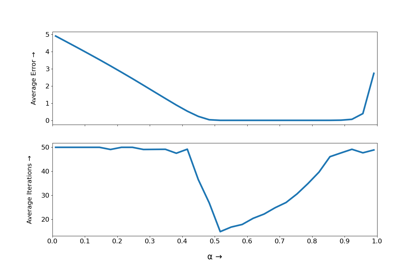
Graph Interpretation

1. Average Error vs α:

   • The error decreases as \( \alpha \) increases from 0 to about 0.5, reaching a minimum.
   • Then the error starts increasing again as \( \alpha \) approaches 1.

2. Average Iterations vs α:

   • The number of iterations remains mostly constant for \( \alpha \) up to around 0.5.
   • Then it drops significantly, reaching a minimum around \( \alpha = 0.5 \), before increasing again as \( \alpha \) approaches 1.

The optimal \( \alpha \) (where both error is minimized and convergence is faster) seems to be around \( \alpha = 0.5 \)

Mathematical Interpretation

Let's take a look at the range of this general approximation and if it covers the whole range:

Let us represent the smaller divisions by \(l_i\) where:

$$l_i = {L}*{\alpha^i}$$

Now, we can estimate \( r \)(remaining distance) by using combinations of \(l_i\). Therefore,

$$r_{approx} = L \cdot \alpha \pm L \cdot \alpha^2 \pm L \cdot \alpha^3 \pm L \cdot \alpha^4 \cdots$$

The minimum value is attained when all following terms are negative i.e.

$$ \displaylines{\begin{align} \min({r_{approx}}) &= L \cdot \alpha - L \cdot \alpha^2 - L \cdot \alpha^3 - L \cdot \alpha^4 \cdots \\ &= L \cdot \alpha - L \cdot \alpha^2\sum_{n=0}^{\infty} \alpha^{n} \\ &= L \cdot \alpha - L \cdot \alpha^2*\frac{1}{1 - \alpha} \\ &= L \cdot \alpha \cdot \frac{1 - 2\alpha}{1 - \alpha}\end{align}} $$

Now we know that the minimum value that we need to approximate is 0. Therefore we have to solve the inequality:

$$ \frac{L \cdot \alpha \cdot (1 - 2\alpha)}{1 - \alpha} \leq 0 $$

Since \( 0 < \alpha < 1\), it follows that \( 0 < 1 - \alpha < 1\).

The inequality reduces to:

$$ (1 - 2\alpha) \leq 0 $$

Therefore, the solution to the inequality is:

$$ \boxed{\frac{1}{2} \leq \alpha < 1} $$

Since the magnitude of the approximation error at pass \(n\) is limited by the current yardstick length (\(L * \alpha^n\)), a smaller value of \(\alpha\) leads to fewer passes needed to achieve a given accuracy.

Therefore, to maximize efficiency, \(\alpha\) should be minimized (\(\alpha = 0.5\)), meaning the yardstick length should be halved with each pass.

Critical Role of \( \boldsymbol{\alpha} \)

Let's look at the approximation visualization for various α:

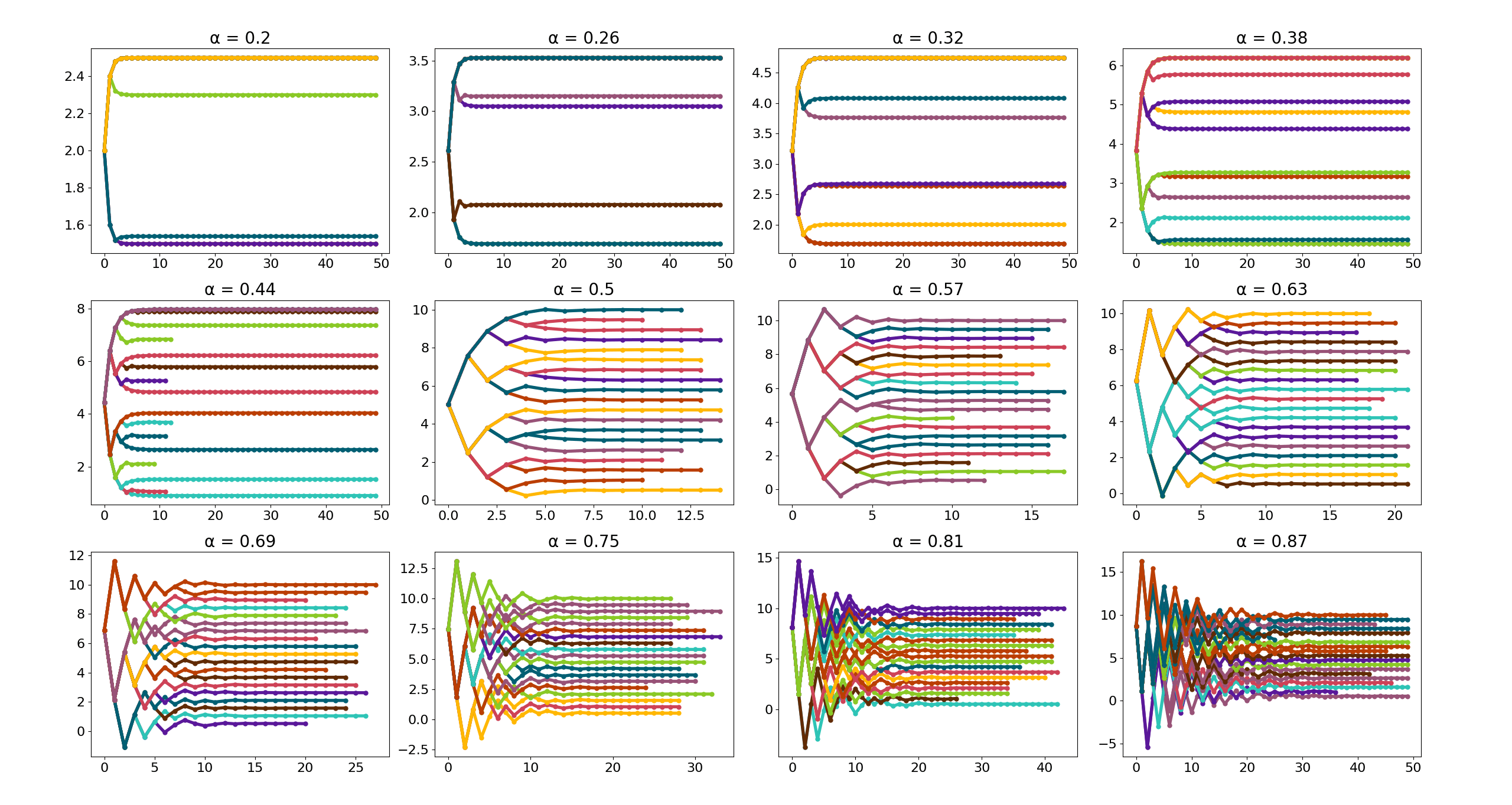
The scaling factor \( \alpha \) directly influences how fast the rope length diminishes with each step. The smaller \( \alpha \) is, the faster the length of the rope reduces.

• \( \boldsymbol{\alpha < 0.5} \): The rope length decreases very quickly, potentially making the series converge too slowly, and in some cases, the approximation process might not adequately capture the remaining distance.

• \( \boldsymbol{\alpha = 0.5} \): The rope length decreases by half at each step. This is a convergent geometric series with a common ratio \( \frac{1}{2} \).

• \( \boldsymbol{\alpha > 0.5} \): The rope length decreases more slowly. The series still converges, but more slowly because the terms decrease less rapidly.

Mission Accomplished ⛵

Utilizing the iterative approximation method, the sailor ingeniously developed a way to measure distances accurately despite the lack of conventional tools. As you consider his resourcefulness and problem-solving skills, I hope you enjoyed assisting him in solving this complex problem and navigating his way back to civilization.

Limitations

While theoretically effective, the successive approximation method using a rope is ultimately limited by the human eye’s visual resolution, the flexibility of the rope, and the cumulative effect of small errors in measurement. These factors make it challenging to achieve high levels of precision, particularly when measuring very small distances.

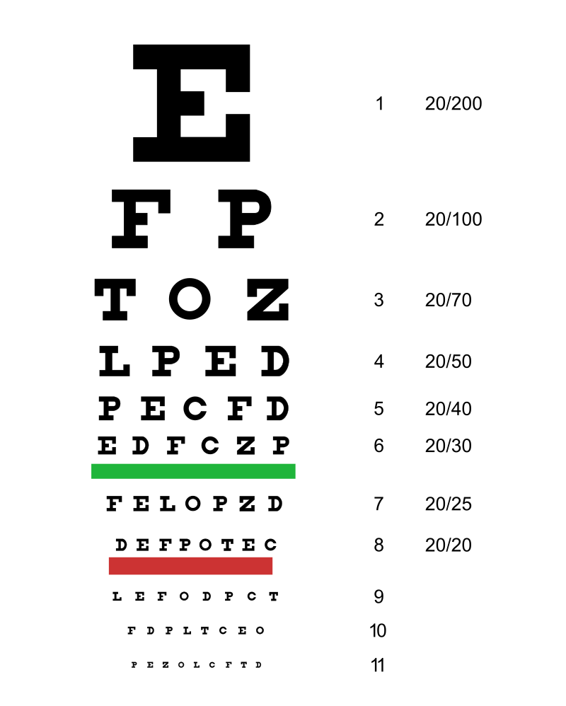
The main limitation being the visual resolution of the eye. The human eye can only perceive differences in position down to about 0.1 to 0.2 millimeters under optimal conditions. This is known as the visual acuity limit.

When attempting to measure small remaining distances by eye, any distance smaller than this limit will be difficult to distinguish. As the rope length is progressively reduced, the remaining error becomes too small for the eye to discern accurately.

General Limitations

Talking about the successive approximation method generally, this algorithm is simple to implement and efficient for moderate precision needs. It handles large ranges and discrete steps, with low computational and memory demands, making it suitable for real-world tasks where exact precision isn't necessary.

While effective in many scenarios, this method has certain limitations. Here are some key limitations:

• Convergence: Slow for some inputs, limited by a fixed number of iterations.
• Precision: Dependent on a fixed error threshold, which may not be ideal for all situations.
• Scale: Relies on a fixed scale, which might not be optimal for different ranges of values.
• Floating-Point Precision: Limited precision when dealing with very large or very small values.
• Complexity: Not suitable for problems requiring high precision, multi-dimensional spaces, or non-smooth functions.

Despite these limitations, this method is still useful in specific contexts where approximate values are acceptable and precision requirements are not too stringent. For more complex cases, more sophisticated techniques may be necessary.

Broader Implications

The iterative approximation methods seen here could be applied in any scenario where:

• A precise value needs to be approximated with predefined units or tolerances.
• Efficiency and simplicity are prioritized over absolute precision.
• Systems must operate within resource constraints or rounding errors, like in hardware devices, video games, and network systems.

The key is that the approximation process ensures you get as close as possible to the desired value without overshooting or unnecessary complexity. The stepwise refinement, especially the diminishing step size, is useful in scenarios where fine-tuned adjustments are needed but with bounds on precision or computational limits.

Analogous Methods

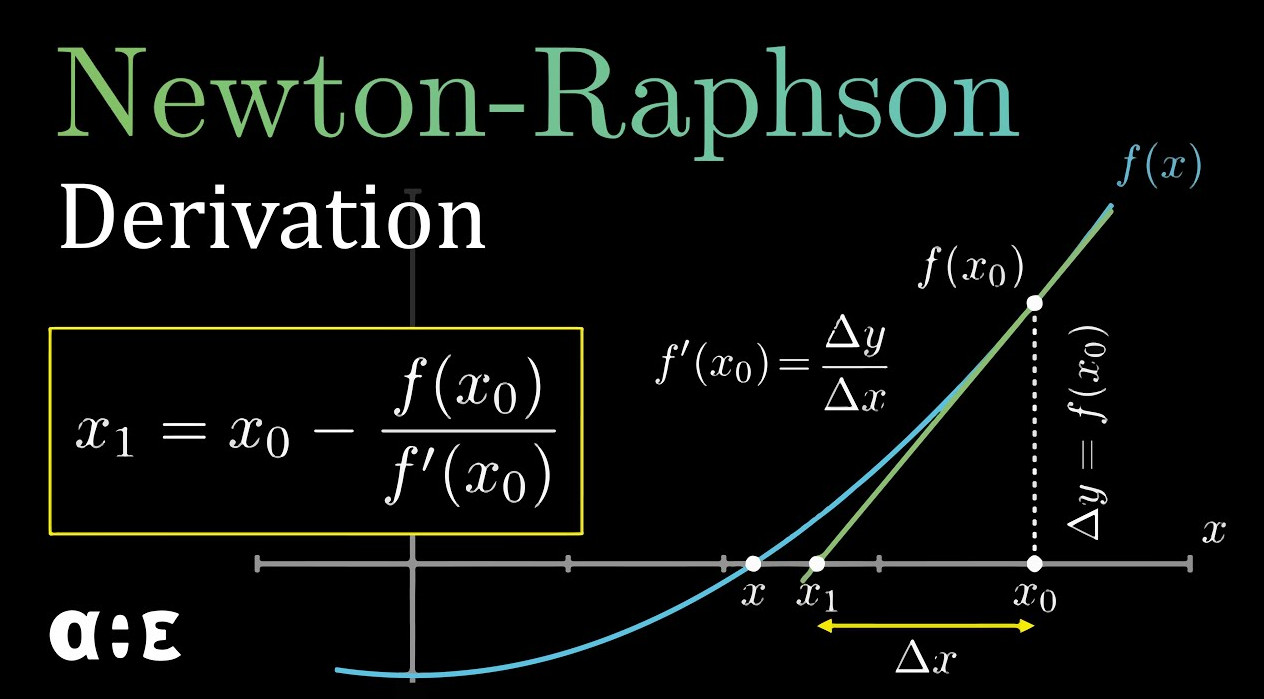
1. Mathematics: Newton-Raphson Method

2. Computer Science: Binary Search

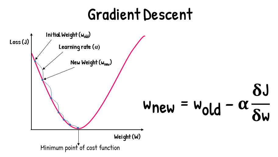
2. Machine Learning: Gradient Descent

3. Electronics: Successive Approximation ADC

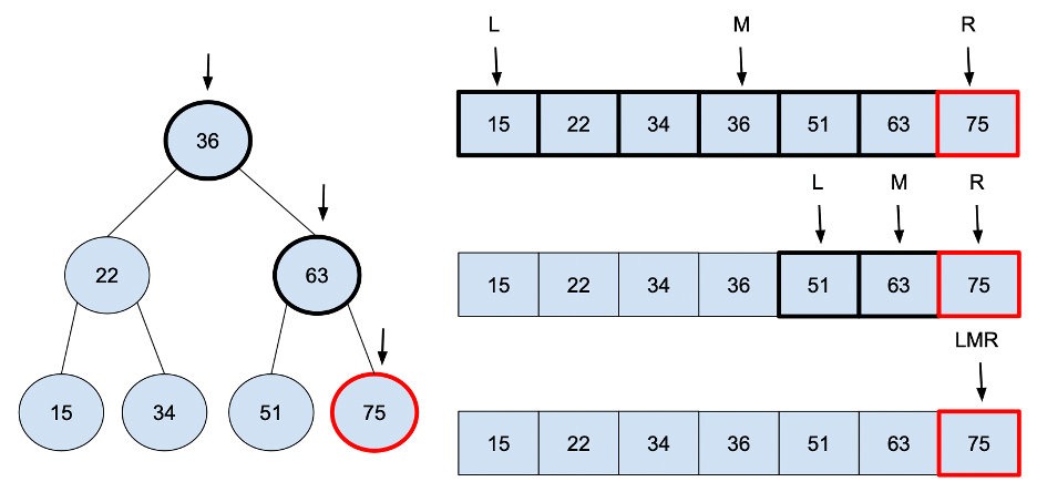
Bonus: Analogy with Binary Search Algorithm

Have you ever wondered why binary search is the most optimal technique for searching a sorted array?

In computer science, binary search, also known as half-interval search, is a search algorithm that finds the position of a target value within a sorted array. It works by dividing the search space in half with each step, reducing the time complexity to \( O(\log n) \), making it far faster than linear search methods.

Now you must be getting to why we halve the search space in binary search rather than reducing it by a factor of, say, 3 or 4. Let's analyze this by looking at the generalized case with the m-ary tree:

m-ary Tree

In graph theory, an m-ary tree (for nonnegative integers m) is an an ordered tree in which each node has no more than m (branching factor) children. This generalizes the concept of binary trees, where each node has at most two children i.e. > m = 2; similarly, a ternary tree is one where m = 3.

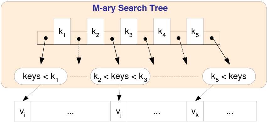
m-ary Search Tree Efficiency

To minimize the number of comparisons in an \( m \)-ary tree, the choice of \( m \) (branching factor) is critical. The goal is to balance the trade-off between the tree's height and the number of comparisons required at each node.

1. Height of the Tree:

   • The height \( h \) of an \( m \)-ary tree with \( N \) end-nodes is given by: $$ \boxed{h = \lceil \log_m N \rceil} $$
   • As \( m \) increases, the height \( h \) decreases which reduces the number of levels you need to traverse.

2. Comparisons at Each Node:

   • At each node, the number of comparisons required is \( m - 1 \), because you need to decide which of the ( m ) children to follow.
   • Larger values of \( m \) reduce the height of the tree but increase the number of comparisons at each node.

Total Comparisons:

The total number of comparisons to traverse the tree is approximately:

$$ \text{Total Comparisons} \approx (m - 1) \times h $$

Substituting \( h = \lceil \log_m N \rceil \):

$$ \boxed{\text{Total Comparisons} \approx (m - 1) \times \lceil \log_m N \rceil} $$

Calculation for \( m = 3 \) and \( N = 1000 \):

• For \( m = 3 \):
  • The height of the tree is approximately \( \log_3 1000 \approx 6.29 \), which rounds up to \( h = 7 \).
  • The number of comparisons per node is \( m - 1 = 2 \) comparisons at each node.

So, the total number of comparisons would be approximately:

$$ \text{Total Comparisons} \approx 7 \times 2 = 14 $$

Calculation for \( m = 2 \) (Binary Tree):

• For \( m = 2 \) (binary tree):
  • The height is \( \log_2 1000 \approx 9.97 \), which rounds up to \( h = 10 \).
  • The number of comparisons per node is \( 1 \), because you compare between two children.

So, the total number of comparisons for a binary tree is:

$$ \text{Total Comparisons} \approx 10 \times 1 = 10 $$

Conclusion:

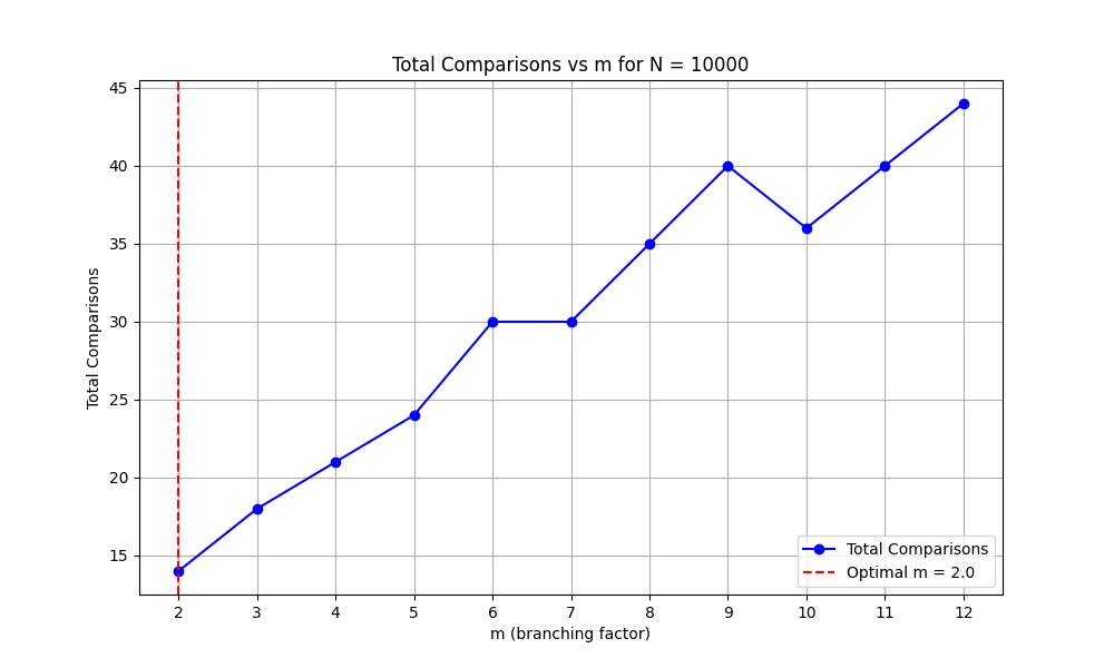
The increase in \( m \) helps reduce height but doesn't necessarily result in fewer total comparisons due to the higher number of comparisons per node. This emphasizes that binary trees often remain optimal in terms of minimizing the total number of comparisons.

In some scenarios like large databases, where time to read the data far exceeds the time needed to compare keys the m-ary search tree might shine. Read more about B-tree.

References

1. E. A.B. Da Silva, D. G. Sampson, and M. Ghanbari. 1996. A successive approximation vector quantizer for wavelet transform image coding
2. Successive-approximation ADC - Wikipedia
3. History of measurement - Wikipedia
4. Numerical analysis - Wikipedia
5. Convergent series - Wikipedia
6. plot(x, y) — Matplotlib 3.9.2 documentation
7. Quickstart - Manim Community v0.18.1

Stay Tuned

Hope you enjoyed reading this. Stay tuned for more cool stuff coming your way!

Dedicated to AJ,

Your encouragement made this possible. Thank you for pushing me to find my voice and for being my constant source of inspiration. This is for you.